Compiler Design

Computers are a balanced mix of software and hardware. Hardware is just a piece of mechanical device and its functions are being controlled by a compatible software. Hardware understands instructions in the form of electronic charge, which is the counterpart of binary language in software programming. Binary language has only two alphabets, 0 and 1. To instruct, the hardware codes must be written in binary format, which is simply a series of 1s and 0s. It would be a difficult and cumbersome task for computer programmers to write such codes, which is why we have compilers to write such codes.

Language Processing System

We have learnt that any computer system is made of hardware and software. The hardware understands a language, which humans cannot understand. So we write programs in high-level language, which is easier for us to understand and remember. These programs are then fed into a series of tools and OS components to get the desired code that can be used by the machine. This is known as Language Processing System.

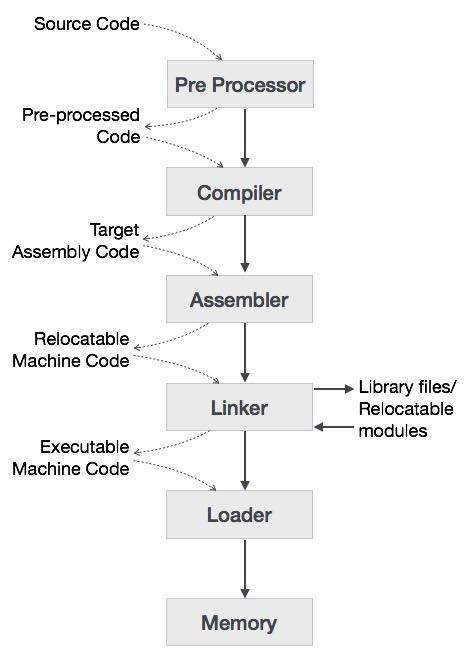
The high-level language is converted into binary language in various phases. A compiler is a program that converts high-level language to assembly language. Similarly, an assembler is a program that converts the assembly language to machine-level language.

Let us first understand how a program, using C compiler, is executed on a host machine.

• User writes a program in C language (high-level language).
• The C compiler, compiles the program and translates it to assembly program (low-level language).
• An assembler then translates the assembly program into machine code (object).
• A linker tool is used to link all the parts of the program together for execution (executable machine code).
• A loader loads all of them into memory and then the program is executed.

Before diving straight into the concepts of compilers, we should understand a few other tools that work closely with compilers.

Preprocessor

A preprocessor, generally considered as a part of compiler, is a tool that produces input for compilers. It deals with macro-processing, augmentation, file inclusion, language extension, etc.

Interpreter

An interpreter, like a compiler, translates high-level language into low-level machine language. The difference lies in the way they read the source code or input. A compiler reads the whole source code at once, creates tokens, checks semantics, generates intermediate code, executes the whole program and may involve many passes. In contrast, an interpreter reads a statement from the input, converts it to an intermediate code, executes it, then takes the next statement in sequence. If an error occurs, an interpreter stops execution and reports it. whereas a compiler reads the whole program even if it encounters several errors.

Assembler

An assembler translates assembly language programs into machine code.The output of an assembler is called an object file, which contains a combination of machine instructions as well as the data required to place these instructions in memory.

Linker

Linker is a computer program that links and merges various object files together in order to make an executable file. All these files might have been compiled by separate assemblers. The major task of a linker is to search and locate referenced module/routines in a program and to determine the memory location where these codes will be loaded, making the program instruction to have absolute references.

Loader

Loader is a part of operating system and is responsible for loading executable files into memory and execute them. It calculates the size of a program (instructions and data) and creates memory space for it. It initializes various registers to initiate execution.

Cross-compiler

A compiler that runs on platform (A) and is capable of generating executable code for platform (B) is called a cross-compiler.

Source-to-source Compiler

A compiler that takes the source code of one programming language and translates it into the source code of another programming language is called a source-to-source compiler.

Compiler Architecture

A compiler can broadly be divided into two phases based on the way they compile.

Analysis Phase

Known as the front-end of the compiler, the analysis phase of the compiler reads the source program, divides it into core parts and then checks for lexical, grammar and syntax errors.The analysis phase generates an intermediate representation of the source program and symbol table, which should be fed to the Synthesis phase as input.

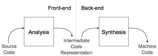
Synthesis Phase

Known as the back-end of the compiler, the synthesis phase generates the target program with the help of intermediate source code representation and symbol table.

A compiler can have many phases and passes.

• Pass : A pass refers to the traversal of a compiler through the entire program.
• Phase : A phase of a compiler is a distinguishable stage, which takes input from the previous stage, processes and yields output that can be used as input for the next stage. A pass can have more than one phase.

Phases of Compiler

The compilation process is a sequence of various phases. Each phase takes input from its previous stage, has its own representation of source program, and feeds its output to the next phase of the compiler. Let us understand the phases of a compiler.

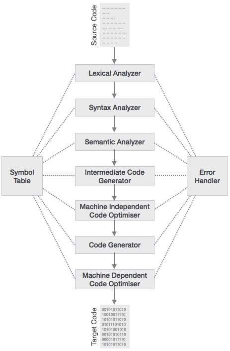
Lexical Analysis

The first phase of scanner works as a text scanner. This phase scans the source code as a stream of characters and converts it into meaningful lexemes. Lexical analyzer represents these lexemes in the form of tokens as:

<token-name, attribute-value>

Syntax Analysis

The next phase is called the syntax analysis or parsing. It takes the token produced by lexical analysis as input and generates a parse tree (or syntax tree). In this phase, token arrangements are checked against the source code grammar, i.e. the parser checks if the expression made by the tokens is syntactically correct.

Semantic Analysis

Semantic analysis checks whether the parse tree constructed follows the rules of language. For example, assignment of values is between compatible data types, and adding string to an integer. Also, the semantic analyzer keeps track of identifiers, their types and expressions; whether identifiers are declared before use or not etc. The semantic analyzer produces an annotated syntax tree as an output.

Intermediate Code Generation

After semantic analysis the compiler generates an intermediate code of the source code for the target machine. It represents a program for some abstract machine. It is in between the high-level language and the machine language. This intermediate code should be generated in such a way that it makes it easier to be translated into the target machine code.

Code Optimization

The next phase does code optimization of the intermediate code. Optimization can be assumed as something that removes unnecessary code lines, and arranges the sequence of statements in order to speed up the program execution without wasting resources (CPU, memory).

Code Generation

In this phase, the code generator takes the optimized representation of the intermediate code and maps it to the target machine language. The code generator translates the intermediate code into a sequence of (generally) re-locatable machine code. Sequence of instructions of machine code performs the task as the intermediate code would do.

Symbol Table

It is a data-structure maintained throughout all the phases of a compiler. All the identifier's names along with their types are stored here. The symbol table makes it easier for the compiler to quickly search the identifier record and retrieve it. The symbol table is also used for scope management.

Compiler Design - Lexical Analysis

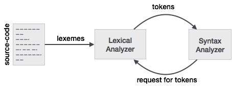
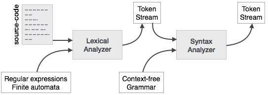
Lexical analysis is the first phase of a compiler. It takes the modified source code from language preprocessors that are written in the form of sentences. The lexical analyzer breaks these syntaxes into a series of tokens, by removing any whitespace or comments in the source code.

If the lexical analyzer finds a token invalid, it generates an error. The lexical analyzer works closely with the syntax analyzer. It reads character streams from the source code, checks for legal tokens, and passes the data to the syntax analyzer when it demands.

Tokens

Lexemes are said to be a sequence of characters (alphanumeric) in a token. There are some predefined rules for every lexeme to be identified as a valid token. These rules are defined by grammar rules, by means of a pattern. A pattern explains what can be a token, and these patterns are defined by means of regular expressions.

In programming language, keywords, constants, identifiers, strings, numbers, operators and punctuations symbols can be considered as tokens.

For example, in C language, the variable declaration line

int value = 100;

contains the tokens:

int (keyword), value (identifier), = (operator), 100 (constant) and ; (symbol).

Specifications of Tokens

Let us understand how the language theory undertakes the following terms:

Alphabets

Any finite set of symbols {0,1} is a set of binary alphabets, {0,1,2,3,4,5,6,7,8,9,A,B,C,D,E,F} is a set of Hexadecimal alphabets, {a-z, A-Z} is a set of English language alphabets.

Strings

Any finite sequence of alphabets is called a string. Length of the string is the total number of occurrence of alphabets, e.g., the length of the string tutorialspoint is 14 and is denoted by |tutorialspoint| = 14. A string having no alphabets, i.e. a string of zero length is known as an empty string and is denoted by ε (epsilon).

Special Symbols

A typical high-level language contains the following symbols:-

Arithmetic Symbols	Addition(+), Subtraction(-), Modulo(%), Multiplication(*), Division(/)
Punctuation	Comma(,), Semicolon(;), Dot(.), Arrow(->)
Assignment	=
Special Assignment	+=, /=, *=, -=
Comparison	==, !=, <, <=, >, >=
Preprocessor	#
Location Specifier	&
Logical	&, &&, |, ||, !
Shift Operator	>>, >>>, <<, <<<

Language

A language is considered as a finite set of strings over some finite set of alphabets. Computer languages are considered as finite sets, and mathematically set operations can be performed on them. Finite languages can be described by means of regular expressions.

Regular Expressions

The lexical analyzer needs to scan and identify only a finite set of valid string/token/lexeme that belong to the language in hand. It searches for the pattern defined by the language rules.

Regular expressions have the capability to express finite languages by defining a pattern for finite strings of symbols. The grammar defined by regular expressions is known as regular grammar. The language defined by regular grammar is known as regular language.

Regular expression is an important notation for specifying patterns. Each pattern matches a set of strings, so regular expressions serve as names for a set of strings. Programming language tokens can be described by regular languages. The specification of regular expressions is an example of a recursive definition. Regular languages are easy to understand and have efficient implementation.

There are a number of algebraic laws that are obeyed by regular expressions, which can be used to manipulate regular expressions into equivalent forms.

Operations

The various operations on languages are:

• Union of two languages L and M is written as
  L U M = {s | s is in L or s is in M}
• Concatenation of two languages L and M is written as
  LM = {st | s is in L and t is in M}
• The Kleene Closure of a language L is written as
  L* = Zero or more occurrence of language L.

Notations

If r and s are regular expressions denoting the languages L(r) and L(s), then

• Union : (r)|(s) is a regular expression denoting L(r) U L(s)
• Concatenation : (r)(s) is a regular expression denoting L(r)L(s)
• Kleene closure : (r)* is a regular expression denoting (L(r))*
• (r) is a regular expression denoting L(r)

Precedence and Associativity

• *, concatenation (.), and | (pipe sign) are left associative
• * has the highest precedence
• Concatenation (.) has the second highest precedence.
• | (pipe sign) has the lowest precedence of all.

Representing valid tokens of a language in regular expression

If x is a regular expression, then:

• x* means zero or more occurrence of x.
  i.e., it can generate { e, x, xx, xxx, xxxx, … }
• x+ means one or more occurrence of x.
  i.e., it can generate { x, xx, xxx, xxxx … } or x.x*
• x? means at most one occurrence of x
  i.e., it can generate either {x} or {e}.
[a-z] is all lower-case alphabets of English language.
[A-Z] is all upper-case alphabets of English language.
[0-9] is all natural digits used in mathematics.

Representing occurrence of symbols using regular expressions

letter = [a – z] or [A – Z]

digit = 0 | 1 | 2 | 3 | 4 | 5 | 6 | 7 | 8 | 9 or [0-9]

sign = [ + | - ]

Representing language tokens using regular expressions

Decimal = (sign)^?(digit)⁺

Identifier = (letter)(letter | digit)*

The only problem left with the lexical analyzer is how to verify the validity of a regular expression used in specifying the patterns of keywords of a language. A well-accepted solution is to use finite automata for verification.

Finite Automata

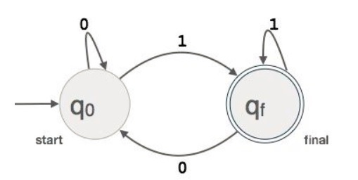
Finite automata is a state machine that takes a string of symbols as input and changes its state accordingly. Finite automata is a recognizer for regular expressions. When a regular expression string is fed into finite automata, it changes its state for each literal. If the input string is successfully processed and the automata reaches its final state, it is accepted, i.e., the string just fed was said to be a valid token of the language in hand.

The mathematical model of finite automata consists of:

• Finite set of states (Q)
• Finite set of input symbols (Σ)
• One Start state (q0)
• Set of final states (qf)
• Transition function (δ)

The transition function (δ) maps the finite set of state (Q) to a finite set of input symbols (Σ), Q × Σ ➔ Q

Finite Automata Construction

Let L(r) be a regular language recognized by some finite automata (FA).

• States : States of FA are represented by circles. State names are written inside circles.
• Start state : The state from where the automata starts, is known as the start state. Start state has an arrow pointed towards it.
• Intermediate states : All intermediate states have at least two arrows; one pointing to and another pointing out from them.
• Final state : If the input string is successfully parsed, the automata is expected to be in this state. Final state is represented by double circles. It may have any odd number of arrows pointing to it and even number of arrows pointing out from it. The number of odd arrows are one greater than even, i.e. odd = even+1.
• Transition : The transition from one state to another state happens when a desired symbol in the input is found. Upon transition, automata can either move to the next state or stay in the same state. Movement from one state to another is shown as a directed arrow, where the arrows points to the destination state. If automata stays on the same state, an arrow pointing from a state to itself is drawn.

Example : We assume FA accepts any three digit binary value ending in digit 1. FA = {Q(q₀, q_f), Σ(0,1), q₀, q_f, δ}

Longest Match Rule

When the lexical analyzer read the source-code, it scans the code letter by letter; and when it encounters a whitespace, operator symbol, or special symbols, it decides that a word is completed.

For example:

int intvalue;

While scanning both lexemes till ‘int’, the lexical analyzer cannot determine whether it is a keyword int or the initials of identifier int value.

The Longest Match Rule states that the lexeme scanned should be determined based on the longest match among all the tokens available.

The lexical analyzer also follows rule priority where a reserved word, e.g., a keyword, of a language is given priority over user input. That is, if the lexical analyzer finds a lexeme that matches with any existing reserved word, it should generate an error.

Compiler Design - Syntax Analysis

Syntax analysis or parsing is the second phase of a compiler. In this chapter, we shall learn the basic concepts used in the construction of a parser.

We have seen that a lexical analyzer can identify tokens with the help of regular expressions and pattern rules. But a lexical analyzer cannot check the syntax of a given sentence due to the limitations of the regular expressions. Regular expressions cannot check balancing tokens, such as parenthesis. Therefore, this phase uses context-free grammar (CFG), which is recognized by push-down automata.

CFG, on the other hand, is a superset of Regular Grammar, as depicted below:

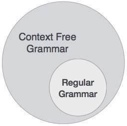
It implies that every Regular Grammar is also context-free, but there exists some problems, which are beyond the scope of Regular Grammar. CFG is a helpful tool in describing the syntax of programming languages.

Context-Free Grammar

In this section, we will first see the definition of context-free grammar and introduce terminologies used in parsing technology.

A context-free grammar has four components:

• A set of non-terminals (V). Non-terminals are syntactic variables that denote sets of strings. The non-terminals define sets of strings that help define the language generated by the grammar.
• A set of tokens, known as terminal symbols (Σ). Terminals are the basic symbols from which strings are formed.
• A set of productions (P). The productions of a grammar specify the manner in which the terminals and non-terminals can be combined to form strings. Each production consists of a non-terminal called the left side of the production, an arrow, and a sequence of tokens and/or on- terminals, called the right side of the production.
• One of the non-terminals is designated as the start symbol (S); from where the production begins.

The strings are derived from the start symbol by repeatedly replacing a non-terminal (initially the start symbol) by the right side of a production, for that non-terminal.

Example

We take the problem of palindrome language, which cannot be described by means of Regular Expression. That is, L = { w | w = w^R } is not a regular language. But it can be described by means of CFG, as illustrated below:

G = ( V, Σ, P, S )

Where:

V = { Q, Z, N }
Σ = { 0, 1 }
P = { Q → Z | Q → N | Q → ℇ | Z → 0Q0 | N → 1Q1 }
S = { Q }

This grammar describes palindrome language, such as: 1001, 11100111, 00100, 1010101, 11111, etc.

Syntax Analyzers

A syntax analyzer or parser takes the input from a lexical analyzer in the form of token streams. The parser analyzes the source code (token stream) against the production rules to detect any errors in the code. The output of this phase is a parse tree.

This way, the parser accomplishes two tasks, i.e., parsing the code, looking for errors and generating a parse tree as the output of the phase.

Parsers are expected to parse the whole code even if some errors exist in the program. Parsers use error recovering strategies, which we will learn later in this chapter.

Derivation

A derivation is basically a sequence of production rules, in order to get the input string. During parsing, we take two decisions for some sentential form of input:

• Deciding the non-terminal which is to be replaced.
• Deciding the production rule, by which, the non-terminal will be replaced.

To decide which non-terminal to be replaced with production rule, we can have two options.

Left-most Derivation

If the sentential form of an input is scanned and replaced from left to right, it is called left-most derivation. The sentential form derived by the left-most derivation is called the left-sentential form.

Right-most Derivation

If we scan and replace the input with production rules, from right to left, it is known as right-most derivation. The sentential form derived from the right-most derivation is called the right-sentential form.

Example

Production rules:

E → E + E
E → E * E
E → id 

Input string: id + id * id

The left-most derivation is:

E → E * E
E → E + E * E
E → id + E * E
E → id + id * E
E → id + id * id

Notice that the left-most side non-terminal is always processed first.

The right-most derivation is:

E → E + E
E → E + E * E
E → E + E * id
E → E + id * id
E → id + id * id

Parse Tree

A parse tree is a graphical depiction of a derivation. It is convenient to see how strings are derived from the start symbol. The start symbol of the derivation becomes the root of the parse tree. Let us see this by an example from the last topic.

We take the left-most derivation of a + b * c

The left-most derivation is:

E → E * E
E → E + E * E
E → id + E * E
E → id + id * E
E → id + id * id

Step 1:

E → E * E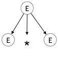

Step 2:

E → E + E * E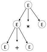

Step 3:

E → id + E * E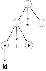

Step 4:

E → id + id * E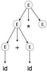

Step 5:

E → id + id * id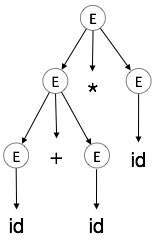

In a parse tree:

• All leaf nodes are terminals.
• All interior nodes are non-terminals.
• In-order traversal gives original input string.

A parse tree depicts associativity and precedence of operators. The deepest sub-tree is traversed first, therefore the operator in that sub-tree gets precedence over the operator which is in the parent nodes.

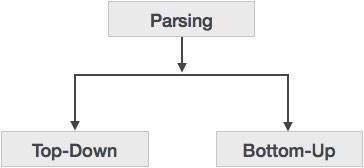
Types of Parsing

Syntax analyzers follow production rules defined by means of context-free grammar. The way the production rules are implemented (derivation) divides parsing into two types : top-down parsing and bottom-up parsing.

Top-down Parsing

When the parser starts constructing the parse tree from the start symbol and then tries to transform the start symbol to the input, it is called top-down parsing.

• Recursive descent parsing : It is a common form of top-down parsing. It is called recursive as it uses recursive procedures to process the input. Recursive descent parsing suffers from backtracking.
• Backtracking : It means, if one derivation of a production fails, the syntax analyzer restarts the process using different rules of same production. This technique may process the input string more than once to determine the right production.

Bottom-up Parsing

As the name suggests, bottom-up parsing starts with the input symbols and tries to construct the parse tree up to the start symbol.

Example:

Input string : a + b * c

Production rules:

S → E
E → E + T
E → E * T
E → T
T → id

Let us start bottom-up parsing

a + b * c

Read the input and check if any production matches with the input:

a + b * c
T + b * c
E + b * c
E + T * c
E * c
E * T
E
S

Ambiguity

A grammar G is said to be ambiguous if it has more than one parse tree (left or right derivation) for at least one string.

Example

E → E + E
E → E – E
E → id

For the string id + id – id, the above grammar generates two parse trees:

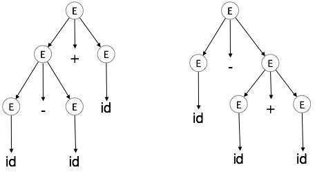
The language generated by an ambiguous grammar is said to be inherently ambiguous. Ambiguity in grammar is not good for a compiler construction. No method can detect and remove ambiguity automatically, but it can be removed by either re-writing the whole grammar without ambiguity, or by setting and following associativity and precedence constraints.

Associativity

If an operand has operators on both sides, the side on which the operator takes this operand is decided by the associativity of those operators. If the operation is left-associative, then the operand will be taken by the left operator or if the operation is right-associative, the right operator will take the operand.

Example

Operations such as Addition, Multiplication, Subtraction, and Division are left associative. If the expression contains:

id op id op id

it will be evaluated as:

(id op id) op id

For example, (id + id) + id

Operations like Exponentiation are right associative, i.e., the order of evaluation in the same expression will be:

id op (id op id)

For example, id ^ (id ^ id)

Precedence

If two different operators share a common operand, the precedence of operators decides which will take the operand. That is, 2+3*4 can have two different parse trees, one corresponding to (2+3)*4 and another corresponding to 2+(3*4). By setting precedence among operators, this problem can be easily removed. As in the previous example, mathematically * (multiplication) has precedence over + (addition), so the expression 2+3*4 will always be interpreted as:

2 + (3 * 4)

These methods decrease the chances of ambiguity in a language or its grammar.

Left Recursion

A grammar becomes left-recursive if it has any non-terminal ‘A’ whose derivation contains ‘A’ itself as the left-most symbol. Left-recursive grammar is considered to be a problematic situation for top-down parsers. Top-down parsers start parsing from the Start symbol, which in itself is non-terminal. So, when the parser encounters the same non-terminal in its derivation, it becomes hard for it to judge when to stop parsing the left non-terminal and it goes into an infinite loop.

Example:

(1) A => Aα | β

(2) S => Aα | β 
    A => Sd 

(1) is an example of immediate left recursion, where A is any non-terminal symbol and α represents a string of non-terminals.

(2) is an example of indirect-left recursion.

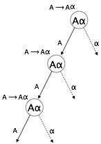
A top-down parser will first parse the A, which in-turn will yield a string consisting of A itself and the parser may go into a loop forever.

Removal of Left Recursion

One way to remove left recursion is to use the following technique:

The production

A => Aα | β

is converted into following productions

A => βA’
A => αA’ | ε

This does not impact the strings derived from the grammar, but it removes immediate left recursion.

Second method is to use the following algorithm, which should eliminate all direct and indirect left recursions.

Algorithm
START
Arrange non-terminals in some order like A1, A2, A3,…, An
for each i from 1 to n
{
for each j from 1 to i-1
   {
   replace each production of form Ai⟹Aj𝜸
   with Ai ⟹ δ1𝜸  | δ2𝜸 | δ3𝜸 |…| 𝜸 
   where Aj ⟹ δ1 | δ2|…| δn  are current Aj productions
}
   }
   eliminate immediate left-recursion
END

Example

The production set

S => Aα | β 
A => Sd

after applying the above algorithm, should become

S => Aα | β 
A => Aαd | βd

and then, remove immediate left recursion using the first technique.

A => βdA’
A => αdA’ | ε

Now none of the production has either direct or indirect left recursion.

Left Factoring

If more than one grammar production rules has a common prefix string, then the top-down parser cannot make a choice as to which of the production it should take to parse the string in hand.

Example

If a top-down parser encounters a production like

A ⟹ αβ | α𝜸 | …

Then it cannot determine which production to follow to parse the string as both productions are starting from the same terminal (or non-terminal). To remove this confusion, we use a technique called left factoring.

Left factoring transforms the grammar to make it useful for top-down parsers. In this technique, we make one production for each common prefixes and the rest of the derivation is added by new productions.

Example

The above productions can be written as

A => αA’
A’=> β | 𝜸 | … 

Now the parser has only one production per prefix which makes it easier to take decisions.

First and Follow Sets

An important part of parser table construction is to create first and follow sets. These sets can provide the actual position of any terminal in the derivation. This is done to create the parsing table where the decision of replacing T[A, t] = α with some production rule.

First Set

This set is created to know what terminal symbol is derived in the first position by a non-terminal. For example,

α → t β

That is α derives t (terminal) in the very first position. So, t ∈ FIRST(α).

ALGORITHM FOR CALCULATING FIRST SET

Look at the definition of FIRST(α) set:

• if α is a terminal, then FIRST(α) = { α }.
• if α is a non-terminal and α → ℇ is a production, then FIRST(α) = { ℇ }.
• if α is a non-terminal and α → 𝜸1 𝜸2 𝜸3 … 𝜸n and any FIRST(𝜸) contains t then t is in FIRST(α).

First set can be seen as: FIRST(α) = { t | α →^* t β } ∪ { ℇ | α →^* ε}

Follow Set

Likewise, we calculate what terminal symbol immediately follows a non-terminal α in production rules. We do not consider what the non-terminal can generate but instead, we see what would be the next terminal symbol that follows the productions of a non-terminal.

ALGORITHM FOR CALCULATING FOLLOW SET:

• if α is a start symbol, then FOLLOW() = $
• if α is a non-terminal and has a production α → AB, then FIRST(B) is in FOLLOW(A) except ℇ.
• if α is a non-terminal and has a production α → AB, where B ℇ, then FOLLOW(A) is in FOLLOW(α).

Follow set can be seen as: FOLLOW(α) = { t | S *αt*}

Error-recovery Strategies

A parser should be able to detect and report any error in the program. It is expected that when an error is encountered, the parser should be able to handle it and carry on parsing the rest of the input. Mostly it is expected from the parser to check for errors but errors may be encountered at various stages of the compilation process. A program may have the following kinds of errors at various stages:

• Lexical : name of some identifier typed incorrectly
• Syntactical : missing semicolon or unbalanced parenthesis
• Semantical : incompatible value assignment
• Logical : code not reachable, infinite loop

There are four common error-recovery strategies that can be implemented in the parser to deal with errors in the code.

Panic mode

When a parser encounters an error anywhere in the statement, it ignores the rest of the statement by not processing input from erroneous input to delimiter, such as semi-colon. This is the easiest way of error-recovery and also, it prevents the parser from developing infinite loops.

Statement mode

When a parser encounters an error, it tries to take corrective measures so that the rest of inputs of statement allow the parser to parse ahead. For example, inserting a missing semicolon, replacing comma with a semicolon etc. Parser designers have to be careful here because one wrong correction may lead to an infinite loop.

Error productions

Some common errors are known to the compiler designers that may occur in the code. In addition, the designers can create augmented grammar to be used, as productions that generate erroneous constructs when these errors are encountered.

Global correction

The parser considers the program in hand as a whole and tries to figure out what the program is intended to do and tries to find out a closest match for it, which is error-free. When an erroneous input (statement) X is fed, it creates a parse tree for some closest error-free statement Y. This may allow the parser to make minimal changes in the source code, but due to the complexity (time and space) of this strategy, it has not been implemented in practice yet.

Abstract Syntax Trees

Parse tree representations are not easy to be parsed by the compiler, as they contain more details than actually needed. Take the following parse tree as an example:

If watched closely, we find most of the leaf nodes are single child to their parent nodes. This information can be eliminated before feeding it to the next phase. By hiding extra information, we can obtain a tree as shown below:

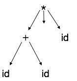
Abstract tree can be represented as:

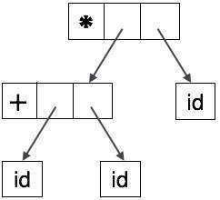
ASTs are important data structures in a compiler with least unnecessary information. ASTs are more compact than a parse tree and can be easily used by a compiler.

Limitations of Syntax Analyzers

Syntax analyzers receive their inputs, in the form of tokens, from lexical analyzers. Lexical analyzers are responsible for the validity of a token supplied by the syntax analyzer. Syntax analyzers have the following drawbacks:

• it cannot determine if a token is valid,
• it cannot determine if a token is declared before it is being used,
• it cannot determine if a token is initialized before it is being used,
• it cannot determine if an operation performed on a token type is valid or not.

These tasks are accomplished by the semantic analyzer, which we shall study in Semantic Analysis.

Compiler Design - Semantic Analysis

We have learnt how a parser constructs parse trees in the syntax analysis phase. The plain parse-tree constructed in that phase is generally of no use for a compiler, as it does not carry any information of how to evaluate the tree. The productions of context-free grammar, which makes the rules of the language, do not accommodate how to interpret them.

For example

E → E + T

The above CFG production has no semantic rule associated with it, and it cannot help in making any sense of the production.

Semantics

Semantics of a language provide meaning to its constructs, like tokens and syntax structure. Semantics help interpret symbols, their types, and their relations with each other. Semantic analysis judges whether the syntax structure constructed in the source program derives any meaning or not.

CFG + semantic rules = Syntax Directed Definitions

For example:

int a = “value”;

should not issue an error in lexical and syntax analysis phase, as it is lexically and structurally correct, but it should generate a semantic error as the type of the assignment differs. These rules are set by the grammar of the language and evaluated in semantic analysis. The following tasks should be performed in semantic analysis:

• Scope resolution
• Type checking
• Array-bound checking

Semantic Errors

We have mentioned some of the semantics errors that the semantic analyzer is expected to recognize:

• Type mismatch
• Undeclared variable
• Reserved identifier misuse.
• Multiple declaration of variable in a scope.
• Accessing an out of scope variable.
• Actual and formal parameter mismatch.

Attribute Grammar

Attribute grammar is a special form of context-free grammar where some additional information (attributes) are appended to one or more of its non-terminals in order to provide context-sensitive information. Each attribute has well-defined domain of values, such as integer, float, character, string, and expressions.

Attribute grammar is a medium to provide semantics to the context-free grammar and it can help specify the syntax and semantics of a programming language. Attribute grammar (when viewed as a parse-tree) can pass values or information among the nodes of a tree.

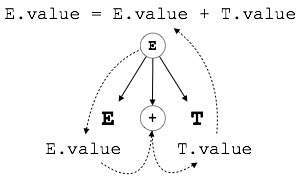
Example:

E → E + T { E.value = E.value + T.value }

The right part of the CFG contains the semantic rules that specify how the grammar should be interpreted. Here, the values of non-terminals E and T are added together and the result is copied to the non-terminal E.

Semantic attributes may be assigned to their values from their domain at the time of parsing and evaluated at the time of assignment or conditions. Based on the way the attributes get their values, they can be broadly divided into two categories : synthesized attributes and inherited attributes.

Synthesized attributes

These attributes get values from the attribute values of their child nodes. To illustrate, assume the following production:

S → ABC

If S is taking values from its child nodes (A,B,C), then it is said to be a synthesized attribute, as the values of ABC are synthesized to S.

As in our previous example (E → E + T), the parent node E gets its value from its child node. Synthesized attributes never take values from their parent nodes or any sibling nodes.

Inherited attributes

In contrast to synthesized attributes, inherited attributes can take values from parent and/or siblings. As in the following production,

S → ABC

A can get values from S, B and C. B can take values from S, A, and C. Likewise, C can take values from S, A, and B.

Expansion : When a non-terminal is expanded to terminals as per a grammatical rule

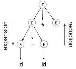
Reduction : When a terminal is reduced to its corresponding non-terminal according to grammar rules. Syntax trees are parsed top-down and left to right. Whenever reduction occurs, we apply its corresponding semantic rules (actions).

Semantic analysis uses Syntax Directed Translations to perform the above tasks.

Semantic analyzer receives AST (Abstract Syntax Tree) from its previous stage (syntax analysis).

Semantic analyzer attaches attribute information with AST, which are called Attributed AST.

Attributes are two tuple value, <attribute name, attribute value>

For example:

int value  = 5;
<type, “integer”>
<presentvalue, “5”>

For every production, we attach a semantic rule.

S-attributed SDT

If an SDT uses only synthesized attributes, it is called as S-attributed SDT. These attributes are evaluated using S-attributed SDTs that have their semantic actions written after the production (right hand side).

As depicted above, attributes in S-attributed SDTs are evaluated in bottom-up parsing, as the values of the parent nodes depend upon the values of the child nodes.

L-attributed SDT

This form of SDT uses both synthesized and inherited attributes with restriction of not taking values from right siblings.

In L-attributed SDTs, a non-terminal can get values from its parent, child, and sibling nodes. As in the following production

S → ABC

S can take values from A, B, and C (synthesized). A can take values from S only. B can take values from S and A. C can get values from S, A, and B. No non-terminal can get values from the sibling to its right.

Attributes in L-attributed SDTs are evaluated by depth-first and left-to-right parsing manner.

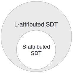
We may conclude that if a definition is S-attributed, then it is also L-attributed as L-attributed definition encloses S-attributed definitions.

Compiler Design - Parser

In the previous chapter, we understood the basic concepts involved in parsing. In this chapter, we will learn the various types of parser construction methods available.

Parsing can be defined as top-down or bottom-up based on how the parse-tree is constructed.

Top-Down Parsing

We have learnt in the last chapter that the top-down parsing technique parses the input, and starts constructing a parse tree from the root node gradually moving down to the leaf nodes. The types of top-down parsing are depicted below:

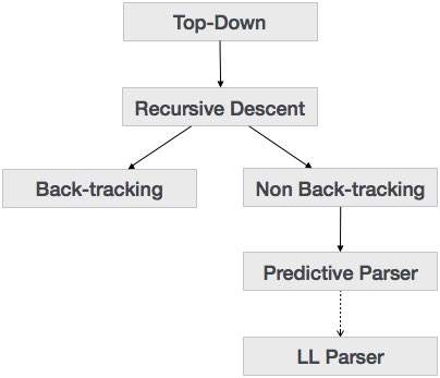
Recursive Descent Parsing

Recursive descent is a top-down parsing technique that constructs the parse tree from the top and the input is read from left to right. It uses procedures for every terminal and non-terminal entity. This parsing technique recursively parses the input to make a parse tree, which may or may not require back-tracking. But the grammar associated with it (if not left factored) cannot avoid back-tracking. A form of recursive-descent parsing that does not require any back-tracking is known as predictive parsing.

This parsing technique is regarded recursive as it uses context-free grammar which is recursive in nature.

Back-tracking

Top- down parsers start from the root node (start symbol) and match the input string against the production rules to replace them (if matched). To understand this, take the following example of CFG:

S → rXd | rZd
X → oa | ea
Z → ai

For an input string: read, a top-down parser, will behave like this:

It will start with S from the production rules and will match its yield to the left-most letter of the input, i.e. ‘r’. The very production of S (S → rXd) matches with it. So the top-down parser advances to the next input letter (i.e. ‘e’). The parser tries to expand non-terminal ‘X’ and checks its production from the left (X → oa). It does not match with the next input symbol. So the top-down parser backtracks to obtain the next production rule of X, (X → ea).

Now the parser matches all the input letters in an ordered manner. The string is accepted.

Predictive Parser

Predictive parser is a recursive descent parser, which has the capability to predict which production is to be used to replace the input string. The predictive parser does not suffer from backtracking.

To accomplish its tasks, the predictive parser uses a look-ahead pointer, which points to the next input symbols. To make the parser back-tracking free, the predictive parser puts some constraints on the grammar and accepts only a class of grammar known as LL(k) grammar.

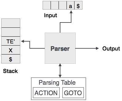
Predictive parsing uses a stack and a parsing table to parse the input and generate a parse tree. Both the stack and the input contains an end symbol $to denote that the stack is empty and the input is consumed. The parser refers to the parsing table to take any decision on the input and stack element combination.

In recursive descent parsing, the parser may have more than one production to choose from for a single instance of input, whereas in predictive parser, each step has at most one production to choose. There might be instances where there is no production matching the input string, making the parsing procedure to fail.

LL Parser

An LL Parser accepts LL grammar. LL grammar is a subset of context-free grammar but with some restrictions to get the simplified version, in order to achieve easy implementation. LL grammar can be implemented by means of both algorithms namely, recursive-descent or table-driven.

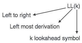
LL parser is denoted as LL(k). The first L in LL(k) is parsing the input from left to right, the second L in LL(k) stands for left-most derivation and k itself represents the number of look aheads. Generally k = 1, so LL(k) may also be written as LL(1).

LL Parsing Algorithm

We may stick to deterministic LL(1) for parser explanation, as the size of table grows exponentially with the value of k. Secondly, if a given grammar is not LL(1), then usually, it is not LL(k), for any given k.

Given below is an algorithm for LL(1) Parsing:

Input: 
string ω 
parsing table M for grammar G
Output:
   If ω is in L(G) then left-most derivation of ω,
   error otherwise.

Initial State : $S on stack (with S being start symbol)
   ω$ in the input buffer

SET ip to point the first symbol of ω$.
repeat
let X be the top stack symbol and a the symbol pointed by ip.
if X∈ Vt or $
if X = a
   POP X and advance ip.
 else
   error()
  endif
else /* X is non-terminal */
   if M[X,a] = X → Y1, Y2,... Yk    
POP X
PUSH Yk, Yk-1,... Y1 /* Y1 on top */
   Output the production X → Y1, Y2,... Yk 
   else
   error()
   endif
 endif
until X = $ /* empty stack */

A grammar G is LL(1) if A-> alpha | b are two distinct productions of G:

• for no terminal, both alpha and beta derive strings beginning with a.
• at most one of alpha and beta can derive empty string.
• if beta=> t, then alpha does not derive any string beginning with a terminal in FOLLOW(A).

Bottom-up Parsing

Bottom-up parsing starts from the leaf nodes of a tree and works in upward direction till it reaches the root node. Here, we start from a sentence and then apply production rules in reverse manner in order to reach the start symbol. The image given below depicts the bottom-up parsers available.

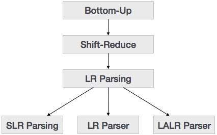
Shift-Reduce Parsing

Shift-reduce parsing uses two unique steps for bottom-up parsing. These steps are known as shift-step and reduce-step.

• Shift step: The shift step refers to the advancement of the input pointer to the next input symbol, which is called the shifted symbol. This symbol is pushed onto the stack. The shifted symbol is treated as a single node of the parse tree.
• Reduce step : When the parser finds a complete grammar rule (RHS) and replaces it to (LHS), it is known as reduce-step. This occurs when the top of the stack contains a handle. To reduce, a POP function is performed on the stack which pops off the handle and replaces it with LHS non-terminal symbol.

LR Parser

The LR parser is a non-recursive, shift-reduce, bottom-up parser. It uses a wide class of context-free grammar which makes it the most efficient syntax analysis technique. LR parsers are also known as LR(k) parsers, where L stands for left-to-right scanning of the input stream; R stands for the construction of right-most derivation in reverse, and k denotes the number of lookahead symbols to make decisions.

There are three widely used algorithms available for constructing an LR parser:

• SLR(1) – Simple LR Parser:
  • Works on smallest class of grammar
  • Few number of states, hence very small table
  • Simple and fast construction
• LR(1) – LR Parser:
  • Works on complete set of LR(1) Grammar
  • Generates large table and large number of states
  • Slow construction
• LALR(1) – Look-Ahead LR Parser:
  • Works on intermediate size of grammar
  • Number of states are same as in SLR(1)

LR Parsing Algorithm

Here we describe a skeleton algorithm of an LR parser:

token = next_token()
repeat forever
   s = top of stack
   if action[s, token] = “shift si” then
   PUSH token
   PUSH si 
   token = next_token()
else if action[s, tpken] = “reduce A::= β“ then 
   POP 2 * |β| symbols
   s = top of stack
   PUSH A
 PUSH goto[s,A]
else if action[s, token] = “accept” then
 return
 else
   error()

LL vs. LR

LL	LR
Does a leftmost derivation.	Does a rightmost derivation in reverse.
Starts with the root nonterminal on the stack.	Ends with the root nonterminal on the stack.
Ends when the stack is empty.	Starts with an empty stack.
Uses the stack for designating what is still to be expected.	Uses the stack for designating what is already seen.
Builds the parse tree top-down.	Builds the parse tree bottom-up.
Continuously pops a nonterminal off the stack, and pushes the corresponding right hand side.	Tries to recognize a right hand side on the stack, pops it, and pushes the corresponding nonterminal.
Expands the non-terminals.	Reduces the non-terminals.
Reads the terminals when it pops one off the stack.	Reads the terminals while it pushes them on the stack.
Pre-order traversal of the parse tree.	Post-order traversal of the parse tree.

Compiler Design - Run-Time Environment

A program as a source code is merely a collection of text (code, statements etc.) and to make it alive, it requires actions to be performed on the target machine. A program needs memory resources to execute instructions. A program contains names for procedures, identifiers etc., that require mapping with the actual memory location at runtime.

By runtime, we mean a program in execution. Runtime environment is a state of the target machine, which may include software libraries, environment variables, etc., to provide services to the processes running in the system.

Runtime support system is a package, mostly generated with the executable program itself and facilitates the process communication between the process and the runtime environment. It takes care of memory allocation and de-allocation while the program is being executed.

Activation Trees

A program is a sequence of instructions combined into a number of procedures. Instructions in a procedure are executed sequentially. A procedure has a start and an end delimiter and everything inside it is called the body of the procedure. The procedure identifier and the sequence of finite instructions inside it make up the body of the procedure.

The execution of a procedure is called its activation. An activation record contains all the necessary information required to call a procedure. An activation record may contain the following units (depending upon the source language used).

Temporaries	Stores temporary and intermediate values of an expression.
Local Data	Stores local data of the called procedure.
Machine Status	Stores machine status such as Registers, Program Counter etc., before the procedure is called.
Control Link	Stores the address of activation record of the caller procedure.
Access Link	Stores the information of data which is outside the local scope.
Actual Parameters	Stores actual parameters, i.e., parameters which are used to send input to the called procedure.
Return Value	Stores return values.

Whenever a procedure is executed, its activation record is stored on the stack, also known as control stack. When a procedure calls another procedure, the execution of the caller is suspended until the called procedure finishes execution. At this time, the activation record of the called procedure is stored on the stack.

We assume that the program control flows in a sequential manner and when a procedure is called, its control is transferred to the called procedure. When a called procedure is executed, it returns the control back to the caller. This type of control flow makes it easier to represent a series of activations in the form of a tree, known as the activation tree.

To understand this concept, we take a piece of code as an example:

. . .
printf(“Enter Your Name: “);
scanf(“%s”, username);
show_data(username);
printf(“Press any key to continue…”);
. . .
int show_data(char *user)
   {
   printf(“Your name is %s”, username);
   return 0;
   }
. . . 

Below is the activation tree of the code given.

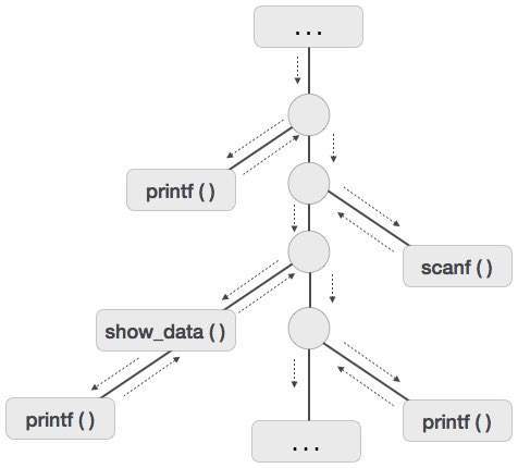
Now we understand that procedures are executed in depth-first manner, thus stack allocation is the best suitable form of storage for procedure activations.

Storage Allocation

Runtime environment manages runtime memory requirements for the following entities:

• Code : It is known as the text part of a program that does not change at runtime. Its memory requirements are known at the compile time.
• Procedures : Their text part is static but they are called in a random manner. That is why, stack storage is used to manage procedure calls and activations.
• Variables : Variables are known at the runtime only, unless they are global or constant. Heap memory allocation scheme is used for managing allocation and de-allocation of memory for variables in runtime.

Static Allocation

In this allocation scheme, the compilation data is bound to a fixed location in the memory and it does not change when the program executes. As the memory requirement and storage locations are known in advance, runtime support package for memory allocation and de-allocation is not required.

Stack Allocation

Procedure calls and their activations are managed by means of stack memory allocation. It works in last-in-first-out (LIFO) method and this allocation strategy is very useful for recursive procedure calls.

Heap Allocation

Variables local to a procedure are allocated and de-allocated only at runtime. Heap allocation is used to dynamically allocate memory to the variables and claim it back when the variables are no more required.

Except statically allocated memory area, both stack and heap memory can grow and shrink dynamically and unexpectedly. Therefore, they cannot be provided with a fixed amount of memory in the system.

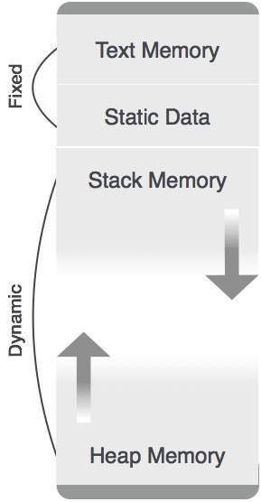
As shown in the image above, the text part of the code is allocated a fixed amount of memory. Stack and heap memory are arranged at the extremes of total memory allocated to the program. Both shrink and grow against each other.

Parameter Passing

The communication medium among procedures is known as parameter passing. The values of the variables from a calling procedure are transferred to the called procedure by some mechanism. Before moving ahead, first go through some basic terminologies pertaining to the values in a program.

r-value

The value of an expression is called its r-value. The value contained in a single variable also becomes an r-value if it appears on the right-hand side of the assignment operator. r-values can always be assigned to some other variable.

l-value

The location of memory (address) where an expression is stored is known as the l-value of that expression. It always appears at the left hand side of an assignment operator.

For example:

day = 1;
week = day * 7;
month = 1;
year = month * 12;

From this example, we understand that constant values like 1, 7, 12, and variables like day, week, month and year, all have r-values. Only variables have l-values as they also represent the memory location assigned to them.

For example:

7 = x + y;

is an l-value error, as the constant 7 does not represent any memory location.

Formal Parameters

Variables that take the information passed by the caller procedure are called formal parameters. These variables are declared in the definition of the called function.

Actual Parameters

Variables whose values or addresses are being passed to the called procedure are called actual parameters. These variables are specified in the function call as arguments.

Example:

fun_one()
{
   int actual_parameter = 10;
   call fun_two(int actual_parameter);
}
   fun_two(int formal_parameter)
{
   print formal_parameter;
}

Formal parameters hold the information of the actual parameter, depending upon the parameter passing technique used. It may be a value or an address.

Pass by Value

In pass by value mechanism, the calling procedure passes the r-value of actual parameters and the compiler puts that into the called procedure’s activation record. Formal parameters then hold the values passed by the calling procedure. If the values held by the formal parameters are changed, it should have no impact on the actual parameters.

Pass by Reference

In pass by reference mechanism, the l-value of the actual parameter is copied to the activation record of the called procedure. This way, the called procedure now has the address (memory location) of the actual parameter and the formal parameter refers to the same memory location. Therefore, if the value pointed by the formal parameter is changed, the impact should be seen on the actual parameter as they should also point to the same value.

Pass by Copy-restore

This parameter passing mechanism works similar to ‘pass-by-reference’ except that the changes to actual parameters are made when the called procedure ends. Upon function call, the values of actual parameters are copied in the activation record of the called procedure. Formal parameters if manipulated have no real-time effect on actual parameters (as l-values are passed), but when the called procedure ends, the l-values of formal parameters are copied to the l-values of actual parameters.

Example:

int y; 
calling_procedure() 
{
   y = 10;     
   copy_restore(y); //l-value of y is passed
   printf y; //prints 99 
}
copy_restore(int x) 
{     
   x = 99; // y still has value 10 (unaffected)
   y = 0; // y is now 0 
}

When this function ends, the l-value of formal parameter x is copied to the actual parameter y. Even if the value of y is changed before the procedure ends, the l-value of x is copied to the l-value of y making it behave like call by reference.

Pass by Name

Languages like Algol provide a new kind of parameter passing mechanism that works like preprocessor in C language. In pass by name mechanism, the name of the procedure being called is replaced by its actual body. Pass-by-name textually substitutes the argument expressions in a procedure call for the corresponding parameters in the body of the procedure so that it can now work on actual parameters, much like pass-by-reference.

Compiler Design - Symbol Table

Symbol table is an important data structure created and maintained by compilers in order to store information about the occurrence of various entities such as variable names, function names, objects, classes, interfaces, etc. Symbol table is used by both the analysis and the synthesis parts of a compiler.

A symbol table may serve the following purposes depending upon the language in hand:

• To store the names of all entities in a structured form at one place.
• To verify if a variable has been declared.
• To implement type checking, by verifying assignments and expressions in the source code are semantically correct.
• To determine the scope of a name (scope resolution).

A symbol table is simply a table which can be either linear or a hash table. It maintains an entry for each name in the following format:

<symbol name,  type,  attribute>

For example, if a symbol table has to store information about the following variable declaration:

static int interest;

then it should store the entry such as:

<interest, int, static>

The attribute clause contains the entries related to the name.

Implementation

If a compiler is to handle a small amount of data, then the symbol table can be implemented as an unordered list, which is easy to code, but it is only suitable for small tables only. A symbol table can be implemented in one of the following ways:

• Linear (sorted or unsorted) list
• Binary Search Tree
• Hash table

Among all, symbol tables are mostly implemented as hash tables, where the source code symbol itself is treated as a key for the hash function and the return value is the information about the symbol.

Operations

A symbol table, either linear or hash, should provide the following operations.

insert()

This operation is more frequently used by analysis phase, i.e., the first half of the compiler where tokens are identified and names are stored in the table. This operation is used to add information in the symbol table about unique names occurring in the source code. The format or structure in which the names are stored depends upon the compiler in hand.

An attribute for a symbol in the source code is the information associated with that symbol. This information contains the value, state, scope, and type about the symbol. The insert() function takes the symbol and its attributes as arguments and stores the information in the symbol table.

For example:

int a;

should be processed by the compiler as:

insert(a, int);

lookup()

lookup() operation is used to search a name in the symbol table to determine:

• if the symbol exists in the table.
• if it is declared before it is being used.
• if the name is used in the scope.
• if the symbol is initialized.
• if the symbol declared multiple times.

The format of lookup() function varies according to the programming language. The basic format should match the following:

lookup(symbol)

This method returns 0 (zero) if the symbol does not exist in the symbol table. If the symbol exists in the symbol table, it returns its attributes stored in the table.

Scope Management

A compiler maintains two types of symbol tables: a global symbol tablewhich can be accessed by all the procedures and scope symbol tables that are created for each scope in the program.

To determine the scope of a name, symbol tables are arranged in hierarchical structure as shown in the example below:

. . . 
int value=10;

void pro_one()
   {
   int one_1;
   int one_2;
   
      {              \
      int one_3;      |_  inner scope 1 
      int one_4;      | 
      }              /
      
   int one_5; 
   
      {              \   
      int one_6;      |_  inner scope 2
      int one_7;      |
      }              /
   }
   
void pro_two()
   {
   int two_1;
   int two_2;
   
      {              \
      int two_3;      |_  inner scope 3
      int two_4;      |
      }              /
      
   int two_5;
   }
. . . 

The above program can be represented in a hierarchical structure of symbol tables:

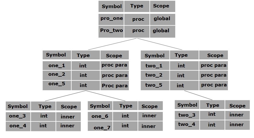
The global symbol table contains names for one global variable (int value) and two procedure names, which should be available to all the child nodes shown above. The names mentioned in the pro_one symbol table (and all its child tables) are not available for pro_two symbols and its child tables.

This symbol table data structure hierarchy is stored in the semantic analyzer and whenever a name needs to be searched in a symbol table, it is searched using the following algorithm:

• first a symbol will be searched in the current scope, i.e. current symbol table.
• if a name is found, then search is completed, else it will be searched in the parent symbol table until,
• either the name is found or global symbol table has been searched for the name.

Compiler - Intermediate Code Generation

A source code can directly be translated into its target machine code, then why at all we need to translate the source code into an intermediate code which is then translated to its target code? Let us see the reasons why we need an intermediate code.

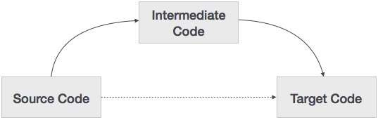
• If a compiler translates the source language to its target machine language without having the option for generating intermediate code, then for each new machine, a full native compiler is required.
• Intermediate code eliminates the need of a new full compiler for every unique machine by keeping the analysis portion same for all the compilers.
• The second part of compiler, synthesis, is changed according to the target machine.
• It becomes easier to apply the source code modifications to improve code performance by applying code optimization techniques on the intermediate code.

Intermediate Representation

Intermediate codes can be represented in a variety of ways and they have their own benefits.

• High Level IR - High-level intermediate code representation is very close to the source language itself. They can be easily generated from the source code and we can easily apply code modifications to enhance performance. But for target machine optimization, it is less preferred.
• Low Level IR - This one is close to the target machine, which makes it suitable for register and memory allocation, instruction set selection, etc. It is good for machine-dependent optimizations.

Intermediate code can be either language specific (e.g., Byte Code for Java) or language independent (three-address code).

Three-Address Code

Intermediate code generator receives input from its predecessor phase, semantic analyzer, in the form of an annotated syntax tree. That syntax tree then can be converted into a linear representation, e.g., postfix notation. Intermediate code tends to be machine independent code. Therefore, code generator assumes to have unlimited number of memory storage (register) to generate code.

For example:

a = b + c * d;

The intermediate code generator will try to divide this expression into sub-expressions and then generate the corresponding code.

r1 = c * d;
r2 = b + r1;
a = r2

r being used as registers in the target program.

A three-address code has at most three address locations to calculate the expression. A three-address code can be represented in two forms : quadruples and triples.

Quadruples

Each instruction in quadruples presentation is divided into four fields: operator, arg1, arg2, and result. The above example is represented below in quadruples format:

Op	arg1	arg2	result
*	c	d	r1
+	b	r1	r2
+	r2	r1	r3
=	r3		a

Triples

Each instruction in triples presentation has three fields : op, arg1, and arg2.The results of respective sub-expressions are denoted by the position of expression. Triples represent similarity with DAG and syntax tree. They are equivalent to DAG while representing expressions.

Op	arg1	arg2
*	c	d
+	b	(0)
+	(1)	(0)
=	(2)

Triples face the problem of code immovability while optimization, as the results are positional and changing the order or position of an expression may cause problems.

Indirect Triples

This representation is an enhancement over triples representation. It uses pointers instead of position to store results. This enables the optimizers to freely re-position the sub-expression to produce an optimized code.

Declarations

A variable or procedure has to be declared before it can be used. Declaration involves allocation of space in memory and entry of type and name in the symbol table. A program may be coded and designed keeping the target machine structure in mind, but it may not always be possible to accurately convert a source code to its target language.

Taking the whole program as a collection of procedures and sub-procedures, it becomes possible to declare all the names local to the procedure. Memory allocation is done in a consecutive manner and names are allocated to memory in the sequence they are declared in the program. We use offset variable and set it to zero {offset = 0} that denote the base address.

The source programming language and the target machine architecture may vary in the way names are stored, so relative addressing is used. While the first name is allocated memory starting from the memory location 0 {offset=0}, the next name declared later, should be allocated memory next to the first one.

Example:

We take the example of C programming language where an integer variable is assigned 2 bytes of memory and a float variable is assigned 4 bytes of memory.

int a;
float b;
Allocation process:
{offset = 0}
int a;
id.type = int
id.width = 2
offset = offset + id.width 
{offset = 2}
float b;
   id.type = float
   id.width = 4
   offset = offset + id.width 
{offset = 6}

To enter this detail in a symbol table, a procedure enter can be used. This method may have the following structure:

enter(name, type, offset)

This procedure should create an entry in the symbol table, for variable name, having its type set to type and relative address offset in its data area.

Compiler Design - Code Generation

Code generation can be considered as the final phase of compilation. Through post code generation, optimization process can be applied on the code, but that can be seen as a part of code generation phase itself. The code generated by the compiler is an object code of some lower-level programming language, for example, assembly language. We have seen that the source code written in a higher-level language is transformed into a lower-level language that results in a lower-level object code, which should have the following minimum properties:

• It should carry the exact meaning of the source code.
• It should be efficient in terms of CPU usage and memory management.

We will now see how the intermediate code is transformed into target object code (assembly code, in this case).

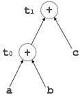
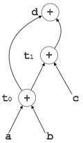
Directed Acyclic Graph

Directed Acyclic Graph (DAG) is a tool that depicts the structure of basic blocks, helps to see the flow of values flowing among the basic blocks, and offers optimization too. DAG provides easy transformation on basic blocks. DAG can be understood here:

• Leaf nodes represent identifiers, names or constants.
• Interior nodes represent operators.
• Interior nodes also represent the results of expressions or the identifiers/name where the values are to be stored or assigned.

Example:

t0 = a + b
t1 = t0 + c
d = t0 + t1

[t0 = a + b]

[t1 = t0 + c]

[d = t0 + t1]

Peephole Optimization

This optimization technique works locally on the source code to transform it into an optimized code. By locally, we mean a small portion of the code block at hand. These methods can be applied on intermediate codes as well as on target codes. A bunch of statements is analyzed and are checked for the following possible optimization:

Redundant instruction elimination

At source code level, the following can be done by the user:

int add_ten(int x) { int y, z; y = 10; z = x + y; return z; }

int add_ten(int x) { int y; y = 10; y = x + y; return y; }

int add_ten(int x) { int y = 10; return x + y; }

int add_ten(int x) { return x + 10; }

At compilation level, the compiler searches for instructions redundant in nature. Multiple loading and storing of instructions may carry the same meaning even if some of them are removed. For example:

• MOV x, R0
• MOV R0, R1

We can delete the first instruction and re-write the sentence as:

MOV x, R1

Unreachable code

Unreachable code is a part of the program code that is never accessed because of programming constructs. Programmers may have accidently written a piece of code that can never be reached.

Example:

void add_ten(int x)
{
   return x + 10;
   printf(“value of x is %d”, x);
}

In this code segment, the printf statement will never be executed as the program control returns back before it can execute, hence printf can be removed.

Flow of control optimization

There are instances in a code where the program control jumps back and forth without performing any significant task. These jumps can be removed. Consider the following chunk of code:

...  
MOV R1, R2
GOTO L1
...
L1 :   GOTO L2
L2 :   INC R1

In this code,label L1 can be removed as it passes the control to L2. So instead of jumping to L1 and then to L2, the control can directly reach L2, as shown below:

...  
MOV R1, R2
GOTO L2
...
L2 :   INC R1

Algebraic expression simplification

There are occasions where algebraic expressions can be made simple. For example, the expression a = a + 0 can be replaced by a itself and the expression a = a + 1 can simply be replaced by INC a.

Strength reduction

There are operations that consume more time and space. Their ‘strength’ can be reduced by replacing them with other operations that consume less time and space, but produce the same result.

For example, x * 2 can be replaced by x << 1, which involves only one left shift. Though the output of a * a and a² is same, a² is much more efficient to implement.

Accessing machine instructions

The target machine can deploy more sophisticated instructions, which can have the capability to perform specific operations much efficiently. If the target code can accommodate those instructions directly, that will not only improve the quality of code, but also yield more efficient results.

Code Generator

A code generator is expected to have an understanding of the target machine’s runtime environment and its instruction set. The code generator should take the following things into consideration to generate the code:

• Target language : The code generator has to be aware of the nature of the target language for which the code is to be transformed. That language may facilitate some machine-specific instructions to help the compiler generate the code in a more convenient way. The target machine can have either CISC or RISC processor architecture.
• IR Type : Intermediate representation has various forms. It can be in Abstract Syntax Tree (AST) structure, Reverse Polish Notation, or 3-address code.
• Selection of instruction : The code generator takes Intermediate Representation as input and converts (maps) it into target machine’s instruction set. One representation can have many ways (instructions) to convert it, so it becomes the responsibility of the code generator to choose the appropriate instructions wisely.
• Register allocation : A program has a number of values to be maintained during the execution. The target machine’s architecture may not allow all of the values to be kept in the CPU memory or registers. Code generator decides what values to keep in the registers. Also, it decides the registers to be used to keep these values.
• Ordering of instructions : At last, the code generator decides the order in which the instruction will be executed. It creates schedules for instructions to execute them.

Descriptors

The code generator has to track both the registers (for availability) and addresses (location of values) while generating the code. For both of them, the following two descriptors are used:

• Register descriptor : Register descriptor is used to inform the code generator about the availability of registers. Register descriptor keeps track of values stored in each register. Whenever a new register is required during code generation, this descriptor is consulted for register availability.
• Address descriptor : Values of the names (identifiers) used in the program might be stored at different locations while in execution. Address descriptors are used to keep track of memory locations where the values of identifiers are stored. These locations may include CPU registers, heaps, stacks, memory or a combination of the mentioned locations.

Code generator keeps both the descriptor updated in real-time. For a load statement, LD R1, x, the code generator:

• updates the Register Descriptor R1 that has value of x and
• updates the Address Descriptor (x) to show that one instance of x is in R1.

Code Generation

Basic blocks comprise of a sequence of three-address instructions. Code generator takes these sequence of instructions as input.

Note : If the value of a name is found at more than one place (register, cache, or memory), the register’s value will be preferred over the cache and main memory. Likewise cache’s value will be preferred over the main memory. Main memory is barely given any preference.

getReg : Code generator uses getReg function to determine the status of available registers and the location of name values. getReg works as follows:

• If variable Y is already in register R, it uses that register.
• Else if some register R is available, it uses that register.
• Else if both the above options are not possible, it chooses a register that requires minimal number of load and store instructions.

For an instruction x = y OP z, the code generator may perform the following actions. Let us assume that L is the location (preferably register) where the output of y OP z is to be saved:

• Call function getReg, to decide the location of L.
• Determine the present location (register or memory) of y by consulting the Address Descriptor of y. If y is not presently in register L, then generate the following instruction to copy the value of y to L:
  MOV y’, L
  where y’ represents the copied value of y.
• Determine the present location of z using the same method used in step 2 for y and generate the following instruction:
  OP z’, L
  where z’ represents the copied value of z.
• Now L contains the value of y OP z, that is intended to be assigned to x. So, if L is a register, update its descriptor to indicate that it contains the value of x. Update the descriptor of x to indicate that it is stored at location L.
• If y and z has no further use, they can be given back to the system.

Other code constructs like loops and conditional statements are transformed into assembly language in general assembly way.

Compiler Design - Code Optimization

Optimization is a program transformation technique, which tries to improve the code by making it consume less resources (i.e. CPU, Memory) and deliver high speed.

In optimization, high-level general programming constructs are replaced by very efficient low-level programming codes. A code optimizing process must follow the three rules given below:

• The output code must not, in any way, change the meaning of the program.
• Optimization should increase the speed of the program and if possible, the program should demand less number of resources.
• Optimization should itself be fast and should not delay the overall compiling process.

Efforts for an optimized code can be made at various levels of compiling the process.

• At the beginning, users can change/rearrange the code or use better algorithms to write the code.
• After generating intermediate code, the compiler can modify the intermediate code by address calculations and improving loops.
• While producing the target machine code, the compiler can make use of memory hierarchy and CPU registers.

Optimization can be categorized broadly into two types : machine independent and machine dependent.

Machine-independent Optimization

In this optimization, the compiler takes in the intermediate code and transforms a part of the code that does not involve any CPU registers and/or absolute memory locations. For example:

do
{
   item = 10;
   value = value + item; 
}while(value<100);

This code involves repeated assignment of the identifier item, which if we put this way:

Item = 10;
do
{
   value = value + item; 
} while(value<100);

should not only save the CPU cycles, but can be used on any processor.

Machine-dependent Optimization

Machine-dependent optimization is done after the target code has been generated and when the code is transformed according to the target machine architecture. It involves CPU registers and may have absolute memory references rather than relative references. Machine-dependent optimizers put efforts to take maximum advantage of memory hierarchy.

Basic Blocks

Source codes generally have a number of instructions, which are always executed in sequence and are considered as the basic blocks of the code. These basic blocks do not have any jump statements among them, i.e., when the first instruction is executed, all the instructions in the same basic block will be executed in their sequence of appearance without losing the flow control of the program.

A program can have various constructs as basic blocks, like IF-THEN-ELSE, SWITCH-CASE conditional statements and loops such as DO-WHILE, FOR, and REPEAT-UNTIL, etc.

Basic block identification

We may use the following algorithm to find the basic blocks in a program:

• Search header statements of all the basic blocks from where a basic block starts:
  • First statement of a program.
  • Statements that are target of any branch (conditional/unconditional).
  • Statements that follow any branch statement.
• Header statements and the statements following them form a basic block.
• A basic block does not include any header statement of any other basic block.

Basic blocks are important concepts from both code generation and optimization point of view.

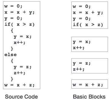
Basic blocks play an important role in identifying variables, which are being used more than once in a single basic block. If any variable is being used more than once, the register memory allocated to that variable need not be emptied unless the block finishes execution.

Control Flow Graph

Basic blocks in a program can be represented by means of control flow graphs. A control flow graph depicts how the program control is being passed among the blocks. It is a useful tool that helps in optimization by help locating any unwanted loops in the program.

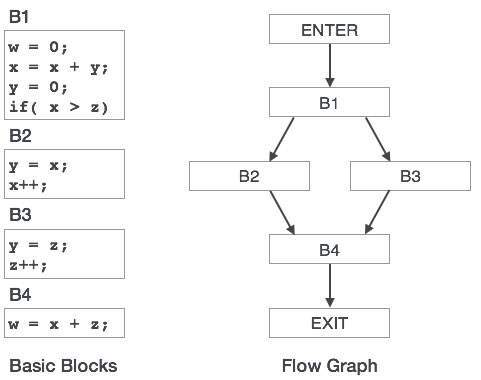
Loop Optimization

Most programs run as a loop in the system. It becomes necessary to optimize the loops in order to save CPU cycles and memory. Loops can be optimized by the following techniques:

• Invariant code : A fragment of code that resides in the loop and computes the same value at each iteration is called a loop-invariant code. This code can be moved out of the loop by saving it to be computed only once, rather than with each iteration.
• Induction analysis : A variable is called an induction variable if its value is altered within the loop by a loop-invariant value.
• Strength reduction : There are expressions that consume more CPU cycles, time, and memory. These expressions should be replaced with cheaper expressions without compromising the output of expression. For example, multiplication (x * 2) is expensive in terms of CPU cycles than (x << 1) and yields the same result.

Dead-code Elimination

Dead code is one or more than one code statements, which are:

• Either never executed or unreachable,
• Or if executed, their output is never used.

Thus, dead code plays no role in any program operation and therefore it can simply be eliminated.

Partially dead code

There are some code statements whose computed values are used only under certain circumstances, i.e., sometimes the values are used and sometimes they are not. Such codes are known as partially dead-code.

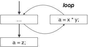
The above control flow graph depicts a chunk of program where variable ‘a’ is used to assign the output of expression ‘x * y’. Let us assume that the value assigned to ‘a’ is never used inside the loop.Immediately after the control leaves the loop, ‘a’ is assigned the value of variable ‘z’, which would be used later in the program. We conclude here that the assignment code of ‘a’ is never used anywhere, therefore it is eligible to be eliminated.

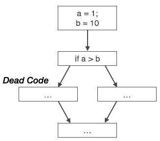
Likewise, the picture above depicts that the conditional statement is always false, implying that the code, written in true case, will never be executed, hence it can be removed.

Partial Redundancy

Redundant expressions are computed more than once in parallel path, without any change in operands.whereas partial-redundant expressions are computed more than once in a path, without any change in operands. For example,

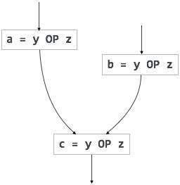
[redundant expression]

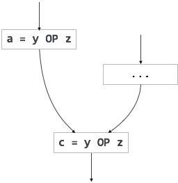
[partially redundant expression]

Loop-invariant code is partially redundant and can be eliminated by using a code-motion technique.

Another example of a partially redundant code can be:

If (condition)
{
   a = y OP z;
}
else
{
   ...
}
c = y OP z;

We assume that the values of operands (y and z) are not changed from assignment of variable a to variable c. Here, if the condition statement is true, then y OP z is computed twice, otherwise once. Code motion can be used to eliminate this redundancy, as shown below:

If (condition)
{
   ...
   tmp = y OP z;
   a = tmp;
   ...
}
else
{
   ...
   tmp = y OP z;
}
c = tmp;

Here, whether the condition is true or false; y OP z should be computed only once.